Month: March 2019

In the last post we used previous day’s minimum and maximum temperatures to forecast tomorrow’s maximum temperature. In this post, we’ll see if we can improve the accuracy of the model using feature engineering. In terms of a benchmark, the Australian Bureau of Meterology published¹ a ‘1 day out’ error of ~1.6^oC while Holmstrom et al² report a ‘1 day out’ RMS error of ~2.8^oC.

We’ve covered the following code in the previous post so we’ll skip through it here, we’re essentially retrieving files and concatenating them into a dataframe. The code block can be expanded by clicking.

library("readr")
library("dplyr")
library("lubridate")

link_address <- "ftp://ftp.bom.gov.au/anon/gen/clim_data/IDCKWCDEA0.tgz"
download.file(link_address, "data/weather.tgz")
untar("data/weather.tgz", exdir = "data/")

weather_readr <- function(file_name = "file name") {
  df_names <- c("Station", "Date", "Etrans", "rain", "Epan", "max_Temp", "min_Temp", "Max_hum", "Min_hum", "Wind", "Rad")
  read.csv(text=paste0(head(readLines(file_name), -1), collapse="\n"), skip = 12, col.names = df_names)
}

file_loc <- "data/tables/vic/melbourne_airport/"
df <- data.frame()
for (files in list.files(file_loc, full.names = TRUE, pattern="*.csv")) {
  dfday <- weather_readr(files)
  df <- rbind(df, dfday)
}

df <- df %>% 
  mutate(Date = dmy(Date))

Pre-processing

In the last post we manually added previous days minimum and maximum temperatures, this time we’ll just create a function, and use it to add the last 2 days of temperature.

library("dplyr")
calc_prev_temps <- function(df_in, n_days) {
  df_in %>% 
    select(Date, max_Temp, min_Temp) %>% 
    mutate(TempMax = lag(max_Temp, n = n_days),
           TempMin = lag(min_Temp, n = n_days)) %>% 
    select(TempMax, TempMin)
}

# loop through the last 7 days
df_input <- df
for (i in 1:7) {
  df_day <- calc_prev_temps(df_input, i)
  df_input <- bind_cols(df_input, df_day)
}

# Exclude non predictor columns
df_input <- df_input %>%  select(-c(1:5,7:11))

Let’s take a look at the data now, the left hand column is “today’s maximum”. The remaining columns are previous maximum and minimum temperature.

max_Temp	TempMax	TempMin	TempMax1	TempMin1
29	29.2	8.1	21.1	6.3
31.7	29	9.7	29.2	8.1
21.4	31.7	13.5	29	9.7
18.4	21.4	15.8	31.7	13.5
19.7	18.4	9.7	21.4	15.8
23.6	19.7	10.2	18.4	9.7

As before we can split the data into a training and test set to build a model and measure it’s accuracy. Last time we used the crude but easily understood Mean Average Error as our accuracy metric, we will report this figure and the Root Mean Squared Error (RMSE) so we may directly compare the results with those of Holmstrom et al.

Modelling

library(h2o)
h2o.init()
hex_df1 <- as.h2o(df_input)
hex_df1 <- h2o.splitFrame(hex_df1) # split into test and training

weather_model <- h2o.gbm(training_frame = hex_df[[1]], y = 1)
h2o.performance(weather_model, hex_df[[2]])

RMSE: 4.09
MAE:  3.05

This is an improvement over our last model. Let’s see if we can improve it more.

Going further

We can extend the function above to include other weather phenomenon; humidity, wind, rain, radiation and evapotranspiration (me neither).

Pre-processing

calc_prev_phen <- function(df_in, n_days) {
  df_in %>% 
    mutate(TempMax = lag(max_Temp, n = n_days),
           TempMin = lag(min_Temp, n = n_days),
           Etrans_lag = lag(Etrans, n = n_days),
           rain_lag = lag(rain, n = n_days),
           Epan_lag = lag(Epan, n = n_days),
           Max_hum_lag = lag(Max_hum, n = n_days),
           Min_hum_lag = lag(Min_hum, n = n_days),
           Wind_nlag = lag(Wind, n = n_days),
           Rad_nlag = lag(Rad, n = n_days)
    ) %>% 
    select(TempMax, TempMin, Etrans_lag, rain_lag, Epan_lag, Max_hum_lag, Min_hum_lag, Wind_nlag, Rad_nlag)
}

As above, we use the function in a loop to build features for the past seven days for each of the phenomenon.

df_input2 <- df
for (i in 1:7) {
  df_day <- calc_prev_phen(df_input2, i)
  df_input2 <- bind_cols(df_input2, df_day)
}

df_input2 <- df_input2 %>%  select(-c(1:5,7:11))

We can preview the data:

Date	max_Temp	TempMax	TempMin	Etrans_lag	rain_lag	Epan_lag	Max_hum_lag	Min_hum_lag	Wind_nlag	Rad_nlag	TempMax1	TempMin1	Etrans_lag1	rain_lag1	Epan_lag1	Max_hum_lag1	Min_hum_lag1	Wind_nlag1	Rad_nlag1
10/01/2009	23.6	19.7	10.2	5.7	0	5.6	79	42	5.37	33.82	18.4	9.7	5.3	0.2	5.2	82	35	7.03	27.48
11/01/2009	23.5	23.6	10.7	5.8	0	7.2	91	45	4.48	32.66	19.7	10.2	5.7	0	5.6	79	42	5.37	33.82
12/01/2009	25.1	23.5	10.7	5.3	0	6.6	90	45	3.89	28.91	23.6	10.7	5.8	0	7.2	91	45	4.48	32.66
13/01/2009	37.1	25.1	10.4	5.4	0	5.2	91	43	3.55	28.02	23.5	10.7	5.3	0	6.6	90	45	3.89	28.91
14/01/2009	33.5	37.1	11.5	11.7	0	6.8	89	8	6.19	34.67	25.1	10.4	5.4	0	5.2	91	43	3.55	28.02

Modelling

Our data set is significantly larger now, but will it increase accuracy?

hex_df2 <- as.h2o(df_input2)
hex_df2 <- h2o.splitFrame(hex_df2) # split into test and training

weather_model2 <- h2o.gbm(training_frame = hex_df2[[1]], y = 1)
h2o.performance(weather_model2, hex_df2[[2]])

RMSE: 3.58
MAE: 2.64

We have squeezed out a little more predictive power from our model, however the predictive error is still larger than the RMSE reported in the literature of ~2.8^oC.

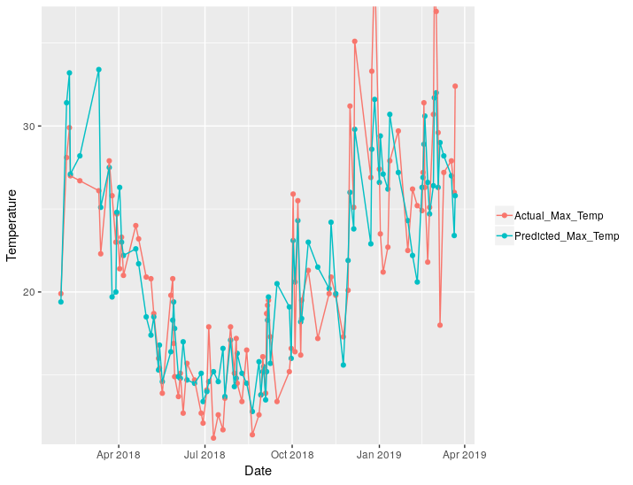
We can plot the actual values against the predicted:

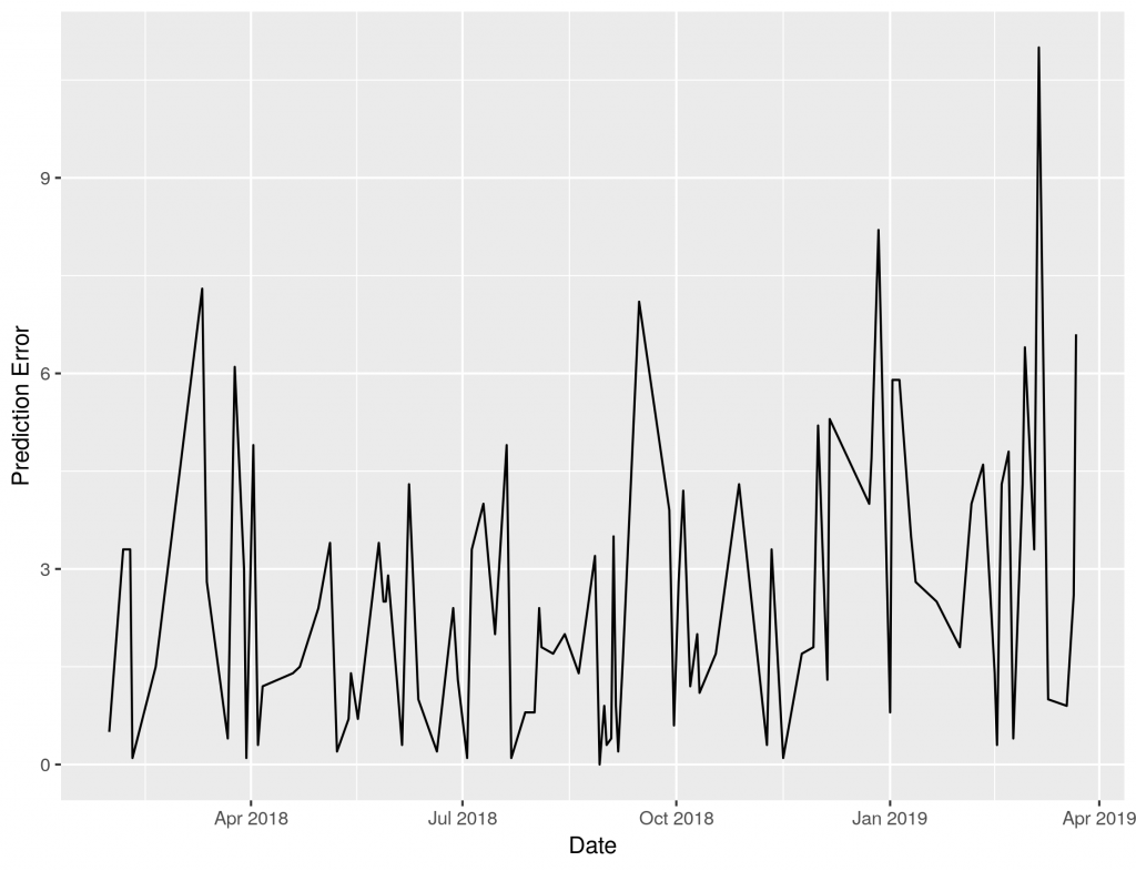
And we can plot just the difference. There is clearly an increase in error in the warmer months, that’s November-March for northern hemispherical readers.

In our next blog, we’ll use one more trick to improve our model.

References

1. Stern, The accuracy of weather forecasts for Melbourne, Australia 2007

2. Holmstrom, Liu, Vo Machine Learning Applied to Weather Forecasting, 2016