Category: Data

In the previous blog we looked at how we could use weather in one location to help predict the weather somewhere else. In this blog we’ll extend this principle, instead of one location we’ll use all weather stations in Victoria. There is no reason why we can’t use weather information from everywhere to predict weather anywhere. Specifically, we’ll look at predicting the next day’s maximum temperature of Melbourne using previous days’ weather across the state.

Introduction

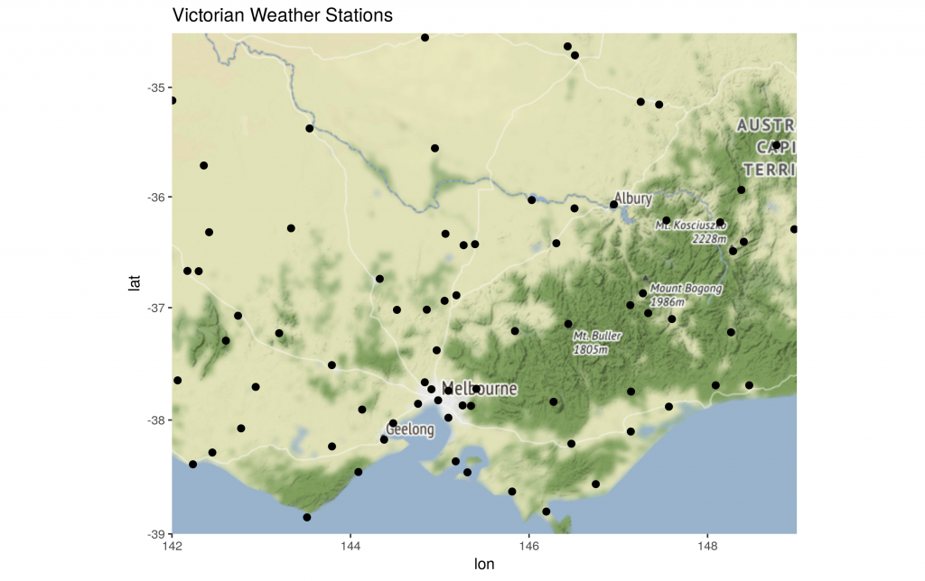
The following map illustrates the locations of BOM weather stations in Victoria, it is a nice grid of sensors sucking up data every day. Each weather station will give us 9 variables (temperature, wind, rain, etc) including our target variable – maximum temperature. If we use several days of previous weather per station, we end up with a very wide dataset. This may be daunting to some that are used to working with a handful of variables, but it is quite manageable.

There is no reason why we can’t use weather information from everywhere to predict weather anywhere

Data Processing

We’ve covered the basic data pipeline in previous blogs so we will skip over them now, but the code can otherwise be exposed below.

# blog 3
library("readr")
library("dplyr")
library("lubridate")

link_address <- "ftp://ftp.bom.gov.au/anon/gen/clim_data/IDCKWCDEA0.tgz"
download.file(link_address, "data/weather.tgz")
untar("data/weather.tgz", exdir = "data/") # this takes a little while
# remove this file
file.remove("data/tables/vic/daily.html")

#----
# Melbourne
weather_readr <- function(file_name = "file name") {
  df_names <- c("Station", "Date",	"Etrans",	"rain",	"Epan", "max_Temp", "min_Temp",	"Max_hum", "Min_hum", "Wind",	"Rad")
  read.csv(text=paste0(head(readLines(file_name), -1), collapse="\n"), skip = 12, col.names = df_names)
}

file_loc <- "data/tables/vic/melbourne_airport/"
df <- data.frame()
for (files in list.files(file_loc, full.names = TRUE, pattern="*.csv")) {
  dfday <- weather_readr(files)
  df <- rbind(df, dfday)
}

As done previously, we’ll use a bunch of variables captured by weather stations. One of the great things about a national weather service is the consistency of data gathered, and being a public service entity, unlikely to change much over many years.

calc_prev_phen <- function(df_in, n_days) {
  df_in %>% 
    mutate(TempMax_nlag = lag(max_Temp, n = n_days),
           TempMin_nlag = lag(min_Temp, n = n_days),
           Etrans_nlag = lag(Etrans, n = n_days),
           rain_nlag = lag(rain, n = n_days),
           Epan_nlag = lag(Epan, n = n_days),
           Max_hum_nlag = lag(Max_hum, n = n_days),
           Min_hum_nlag = lag(Min_hum, n = n_days),
           Wind_nlag = lag(Wind, n = n_days),
           Rad_nlag = lag(Rad, n = n_days),
           
           TempMax_nSum = lag(max_Temp, n = n_days),
           TempMin_nSum = lag(min_Temp, n = n_days)
    ) %>% 
    select(TempMax_nlag, TempMin_nlag, Etrans_nlag, rain_nlag, Epan_nlag, Max_hum_nlag, Min_hum_nlag, Wind_nlag, Rad_nlag, TempMax_nSum, TempMin_nSum)
}

df_melb <- df %>% transmute(Date = dmy(Date), max_Temp_melb = max_Temp)

We use a loop to iterate through all the weather data, which are arranged into monthly files. For simplicity we’ll use just a couple of days here, it does not have a material impact on the accuracy. Feel free to use 7 days, it takes a little longer to run.

for (folders in list.files("../weather/data/tables/vic/")) {
  file_loc <- paste0("../weather/data/tables/vic/", folders) # victorian 
  
  df_input <- data.frame() # loop through each file
  for (files in list.files(file_loc, full.names = TRUE, pattern="*.csv")) {
    dfday <- weather_readr(files)
    df_input <- rbind(df_input, dfday)
  }
  
  df_input <- df_input %>% mutate(Date = dmy(Date))
  
  for (i in 1:2) {
    df_day <- calc_prev_phen(df_input, i)
    df_input <- bind_cols(df_input, df_day)
  }
  
  df_input <- df_input %>% select(-c(1,3:11)) 

  df_melb <- df_melb  %>% left_join(df_input, by = 'Date') 
  
  }

df_melb <- df_melb %>% select(-1) # don't need date field anymore
df_melb <- df_melb %>% select_if(~sum(!is.na(.)) > 1) 

Modelling

We can run the same modelling code as done previously, keeping everything the same.

library(h2o)
h2o.init(nthreads = 1)

hex_df <- as.h2o(df_melb)
hex_df <- h2o.splitFrame(hex_df) # split into test and training

weather_model3 <- h2o.gbm(training_frame = hex_df[[1]], y = 1)
h2o.performance(weather_model3, hex_df[[2]])

We can compare the results of the previous model where we used one location’s weather data, to the current model where we used all Victorian weather station data.

Accuracy Metric	Previous Model (C)	Current Model (C)
MAE	2.64	2.28
RMSE	3.58	3.04

Once again we’ve managed to squeeze out some more accuracy, although ~0.5 degree decrease in average error doesn’t seem like much it does represent ~15% improvement which can be considered significant. More so since there is little extra work required to get attain it. Furthermore, this is a trivial model to build.

Conclusion

Looking back on this series of weather prediction blogs it occurred to me there is a general trend towards replacing deep understanding of a subject with generalised computational techniques that are completely separate from the subject they are describing. A machine learning expert may build an accurate Deep Learning model describing a system despite having no deep understanding of that system.

This may render the data science field into a type of magic, and data scientists will become a type of magician. More worryingly however, it made lead to the demise of technical subject matter experts, and along with it the deep learning of a subject they have acquired. It’s a discussion that’s worth having as the type of technique described above becomes more pervasive.

Appendix

You can generate the map using the code block below.

stations <- read.fwf("data/tables/stations_db.txt",  widths=c(8, 4, 6, 41, 16, 9, 10))
stations <- stations %>% 
  transmute(station = V1, latitude = V6, longitude = V7)

library(ggmap)
location = c( 142.0000, -39.0000, 149.0000, -34.5000)
victoria = get_map(location = location, source = "osm")
victoriaMap <- ggmap(victoria)
victoriaMap + geom_point(data = stations, aes(x = longitude, y = latitude), 
                         size = 2, colour = "black") +
  ggtitle("Victorian Weather Stations")
ggsave("images/weather3.png")